October 19, 2021
Post questions to the Moodle Forum!
In this lab you will apply your knowledge of lists and loops to the task of image processing. First, some background. You can think of a digital image as a large two-dimensional array of pixels, each of which has a red (R) value, a green (G) value, and a blue (B) value. An R, G, or B value is just decimal number between 0 and 1. To modify the image, you need to loop through all of these pixels, one at a time, and do something to some or all of the pixels. For example, to remove all of the green color from each pixel:for every row in the image:
for every column in the image:
set to zero the green value of the pixel in this row and this column The files for this lab are contained in lab5.zip. Download and unzip it to get started. These files are
gray.py: you will modify this file to implement your solution to problem 1 (Grayscale)
blue_screen.py: you will modify this file to implement your solution to problem 2 (Blue Screening)
blur.py: you will modify this file to implement your solution to problem 3 (Blur)
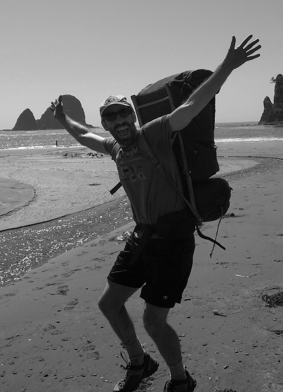
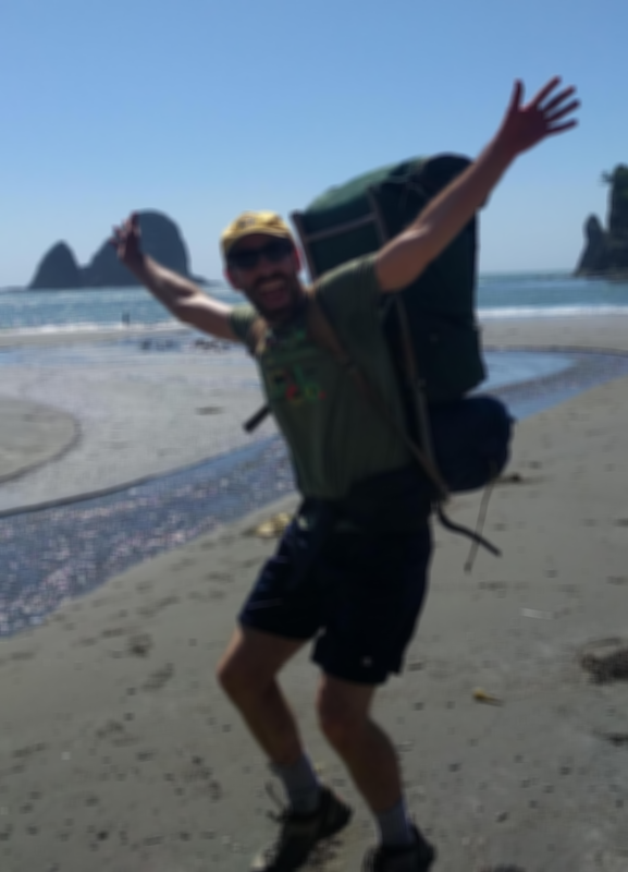
beach_portrait.png: a picture of some backpacking goofball, used as the input image for gray.py
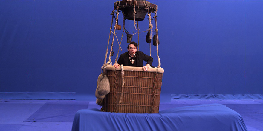
oz_bluescreen.png: a still photo from the set of the 2013 film Oz the Great and Powerful, used as one of the input images for blue_screen.py
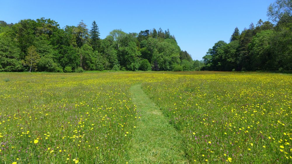
meadow.png: a peaceful meadow scene, used as one of the input images for blue_screen.py
reference-beach_portrait_gray.png: the expected output image for gray.py, provided for your reference
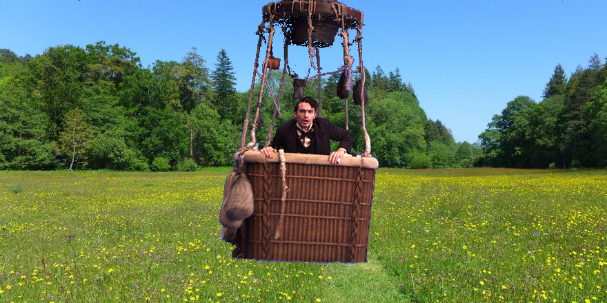
reference-oz_meadow.png: the expected output image for blue_screen.py, provided for your reference
reference-oz_meadow_improved.png: the expected output image for the CHALLENGE improvement to blue_screen.py, provided for your reference
reference-beach_portrait_blur.png: the expected output image for blur.py, provided for your reference
If you look at any of the provided .py files, you will see an unfamiliar import statement: import matplotlib.pyplot as plt. The matplotlib module is what we will use to load, manipulate, and save image data for this homework. The code for loading and saving is already included in the starter files, so you don’t need to write that yourself. What you do need to know is that the function plt.imread, which we use to load image data, returns a 3D array representing the pixel values of that image. An array is very similar to a regular Python list, and you can index and loop over arrays in the same way. Like we saw in class, the 3D array is a list of lists of lists. Thus, the outer list is [row0, row1, row2, ...], each row is [pixel_in_column0, pixel_in_column1, pixel_in_column2, ...], and each pixel is [red_value, green_value, blue_value] (RGB values will be between 0 and 1). You should make sure you understand this structure before starting the lab. Try adding print(image) to gray.py and see if the output makes sense to you. Please post your questions on the Moodle forum or bring them to class.
If you are working on your own computer, you may need to install matplotlib before you can do this homework. Running the command
python3 -m pip install matplotlib
in the terminal should install it. If you’re on Windows, try
py -m pip install matplotlib
Come see me if this doesn’t work.
Suggested Timeline:
Modify gray.py to convert image to a black-and-white or grayscale version of the original. In the RGB color model, gray tones are produced when the values of red, green, and blue are all equal. A simple way to do this conversion is to set the red, green, and blue values for each pixel to the average of those values in the original image. That is \(R_{gray} = G_{gray} = B_{gray} = \frac{R + G + B}{3}\). When you have implemented a correct solution, running gray.py should produce a file called beach_portrat_gray.png that is the same image as reference-beach_portrait_gray.png:
Movies–particularly (non-animated) action movies that use a lot of special effects–often use a technique called blue screening to generate some scenes. The actors in a scene are filmed as they perform in front of a blue screen and, later, the special-effects crew removes the blue from the scene and replaces it with another background (an ocean, a skyline, the Carleton campus). The same technique is used for television weather reports–the meteorologist is not really gesturing at cold fronts and snow storms, just at a blank screen. (Sometimes green screening is used instead; the choice depends on things like the skin tone of the star.) This problem asks you to do something similar.
We can combine an image of, say, James Franco on the set of Oz the Great and Powerful (oz_bluescreen.png) with an image of scenery (meadow.png) by replacing the bluish pixels in the first picture with pixels from a background picture. To do this, we have to figure out which pixels are bluish (and can be changed) and which ones correspond to the actor and props (and should be left alone). Identifying which pixels are sufficiently blue is tricky. Here’s an approach that works reasonably well here: count any pixel that satisfies the following formula as “blue” for the purposes of blue screening: \(B > R + G\).
Modify blue_screen.py to use this formula to replace the appropriate pixels in image with pixels from background. When you have implemented a correct solution, running blue_screen.py should produce a file called oz_meadow.png that is the same image as reference-oz_meadow.png.
 +
+  =
=
Modify blur.py to implement the function blur(img, radius). Your blur function should create and return a blurry version of the image (img). For each pixel, average all of the pixels within a square radius of that pixel. Here’s an example what that means:
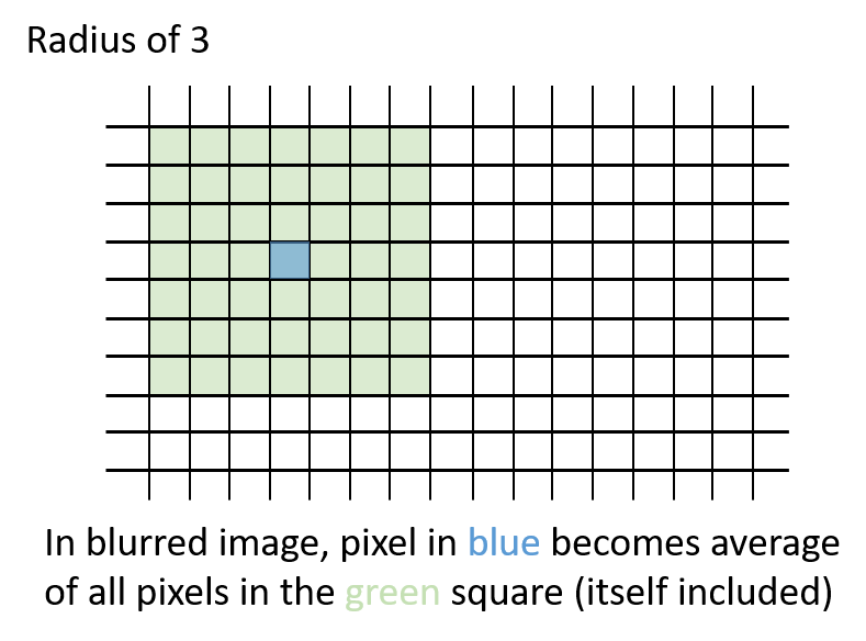
Each pixel will become the average of the square of pixels around it. Pixels at the edges of the image will use whatever part of the square actually exists. Here’s an animation of how the square radius moves with each pixel:
A good way to approach this would be to use radius to slice out a square around the pixel in question. For example, img[0:10, 0:10] would slice out a 10-by-10 square from the upper left corner of the image (note that unlike lists, arrays let us index rows and columns separated by commas instead of multiple sets of brackets). To get the average of the elements of an array you can use .mean() (e.g., img[:, :, 0].mean() would be the average red value for the entire image because it slices out all rows, all columns, and the first element (red) of each pixel).
Make sure to put all of your results in a new image (img.copy() will return a copy of img), instead of overwriting your original as you go; otherwise, your blurred pixels will cascade on top of each other. Be careful near the borders of the image. Keep in mind that some approaches to this problem will result in much slower performance. Any technique that works will receive most of the credit, but your blur.py should run in less than 30 seconds to earn full credit. But do be careful; it’s possible to find solution that take a lot longer!
When you have implemented a correct solution, running blur.py should produce a file called beach_portrait_blur.png that is the same image as reference-beach_portrait_blur.png. Make sure the code you submit calls blur with a radius of 3 like the starter code.
In a file called red_green.py, implement a simplistic simulation of what a red–green colorblind (deuteranopic) viewer would see when looking at the image. To do so, set both the red and green pixel values to be the average of the original red and green pixel values. That way [0.5, 0, 0] and [0, 0.5, 0] will both come out as [0.25, 0.25, 0]. This file should read in beach_portrait.png and produce a new file called beach_portrait_red_green.png.
If you look closely at oz_meadow.png you will notice a number of small errors (sometimes called artifacts). These include bits of blue mixed in with the meadow grasses, a blue outline around the balloon basket, and bits of James Franco replaced with tree pixels. For this challenge, improve the formula used for determining “blue” pixels such that these errors are avoided. Your solution must produce an image at least as good as reference-oz_meadow_improved.png.

In a file called dither.py, write a function dither(image) plus code to test your function. Dithering is a technique used to print a gray picture in a legacy medium (such as a newspaper) where no shades of gray are available. Instead, you need to use individual pixels of black and white to simulate shades of gray. A standard approach to dithering is the Floyd–Steinberg algorithm, which works as follows:
Some tips: (1) Dithering should only be done on grayscale images–actually you can dither color images, too, but it’s more complicated–so use gray.py to convert an image to gray before you get started. (2) In order for dithering to work, you must make your changes to the same image that you are looping over. Dithering by reading one image and making your changes on a copy will not work correctly, because the error never gets a chance to accumulate. In other words, make sure that you make a grayscale copy of the image first, and then do all dithering work (looping, reading, writing, etc.) on the copy itself.
Your best tool for determining the correctness of your output images is the provided reference images. A visual comparison of the two will catch any major differences. To detect bugs that result in minor differences from the expected output, you might consider writing code that uses matplotlib to load both your image and the reference image. You could then write code to compare the values at each pixel of your image to the corresponding pixel in the reference image to check for any differences.
Submit the following files via the Lab 5 Moodle page. You do not need to submit any .png files.
Your modified gray.py, blue_screen.py, and blur.py. If you did the Improved Blue Screening CHALLENGE, note that in comments at the top of blue_screen.py.
OPTIONALLY red-green.py and/or dither.py for the corresponding CHALLENGES
This assignment is graded out of 30 points as follows:
gray.py – 5 points
blue_screen.py – 8 points
blur.py – 10 points
if statements to handle them together inside a single set of nested loops).py file you submit – 1 pointAcknowledgments: This assignment description is modified from previous ones written by David Liben-Nowell.