Hashing II
Table of Contents
1 Reading
Read Sections 15.4.1, 15.4.2, and 15.4.5 of Bailey.
2 Hash Tables: Review
- Aim for constant-time put, contains, and remove
- "On average" under some reasonable assumptions
- A hash table is an array of some fixed size
- But extensible as we'll see
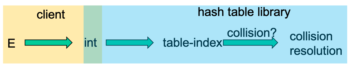
3 Collisions
3.1 Collision Avoidance
- With \(h(x) = x \% \mathrm{size}\) the number of collisions depends on
- the ints inserted (obviously)
- size
- Larger table-size tends to help, but not always
- Example: 70, 24, 56, 43, 10
- same collision with size = 10 and size = 60
- Technique: Pick table size to be prime. Why?
- Real-life data tends to have a pattern
- "Multiples of 61" are probably less likely than "multiples of 60"
3.2 Collision Resolution
3.2.1 Separate Chaining
- Chaining:
- All keys that map to the same table location are kept in a linked list (a.k.a. a chain or bucket)
- As easy as it sounds
- Example: insert 11, 24, 106, 13, 46 with mod hashing and TableSize = 11

- Worst-case time for contains?
- Linear
- But only with really bad luck or bad hash function
- So not worth doing extra work to avoid this worst case
- Beyond asymptotic complexity, some data-structure engineering may be warranted
- Linked list vs. array vs. chunked list (lists should be short!)
- Move-to-front (after every access, move the just accessed node to the front of the linked list, so it will be faster to access next time)
- Maybe leave room for 1 element (or 2?) in the table itself, to optimize constant factors for the common case
- A time-space trade-off…
3.2.2 Load Factor
The load factor λ of a hash table is
\[\lambda = \frac{n}{size}\]
where \(n\) is the number of elements in the hash table.
- Under chaining, the average number of elements per bucket is λ
- So if some puts are followed by random contains, then on average:
- Each unsuccessful contains compares against λ items
- Each successful contains compares against \(\frac{\lambda}{2}\) items
- So we like to keep λ fairly low (e.g., 1 or 1.5 or 2) for chaining
3.2.3 Probing
Alternative idea: use empty space in the table.
- If index \(h(key) \% \mathrm{size}\) is already full,
- try \((h(key) + 1) \% \mathrm{size}\). If full,
- try \((h(key) + 2) \% \mathrm{size}\). If full,
- try \((h(key) + 3) \% \mathrm{size}\). If full…
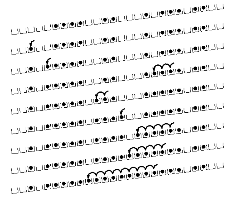
Example: insert 38, 19, 8, 109, 10

This try the next spot approach is called linear probing or open addressing. It turns out to have some problems.
- Tends to produce clusters, which lead to long probing sequences
- Called primary clustering
- Saw this starting in our example
- For any \(\lambda < 1\), linear probing will find an empty slot
- It is safe in this sense: no infinite loop unless table is full
- Linear-probing performance degrades rapidly as table gets full
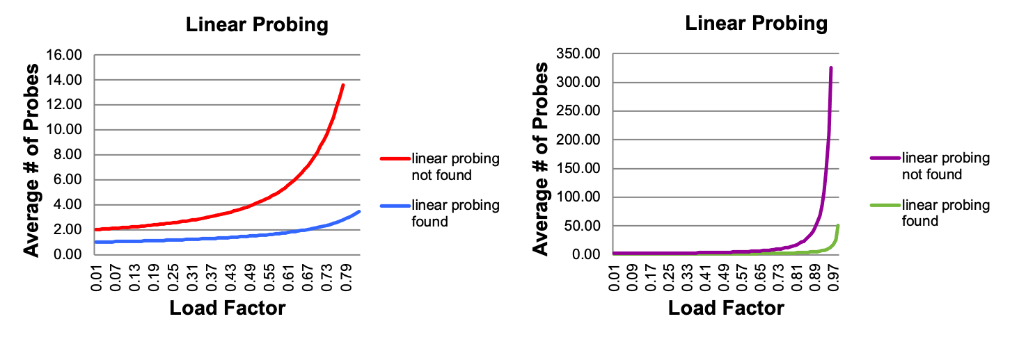
- By comparison, chaining performance is linear in λ and has no trouble with \(\lambda > 1\)
3.2.4 Quadratic Probing
We can avoid primary clustering by changing the probe function \[(h(key) + f(i)) \% \mathrm{size}\]
A common technique is quadratic probing: \[f(i) = i^2\] So probe sequence is:
- 0th probe: \(h(key) \% \mathrm{size}\)
- 1st probe: \((h(key) + 1) \% \mathrm{size}\)
- 2nd probe: \((h(key) + 4) \% \mathrm{size}\)
- 3rd probe: \((h(key) + 9) \% \mathrm{size}\)
- …
- ith probe: \((h(key) + i^2) \% \mathrm{size}\)
Intuition: Probes quickly "leave the neighborhood"

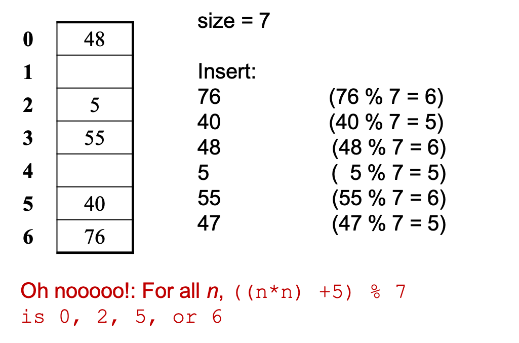
- Bad news:
- Quadratic probing can cycle through the same full indices, never terminating despite table not being full
- Good news:
- If TableSize is prime and \(\lambda < \frac{1}{2}\), then quadratic probing will find an empty slot in at most \(\frac{\mathrm{size}}{2}\) probes
- So: If you keep \(\lambda < \frac{1}{2}\) and size is prime, no need to detect cycles
4 Rehashing
- As with array-based stacks/queues/lists, if table gets too full, create a bigger table and copy everything
- Re-apply the hash function to find the next index for each key
- With chaining, we get to decide what too full means
- Keep load factor reasonable (e.g., < 1)?
- Consider average or max size of non-empty chains?
- For probing, half-full is a good rule of thumb
- New table size
- Twice-as-big is a good idea, except that won't be prime!
- So go about twice-as-big
- Can have a list of prime numbers in your code since you very likely won't grow more than 20-30 times
5 Practice Problems1
- What is the load factor (\(\lambda\)) of a hash table?
- What is a hash collision?
- In a hash table is it possible to have a load factor of 2?
- Is a constant-time performance guaranteed for hash tables?
- What is the final state of a hash table of size 10 after adding 35, 2, 15, 80, 42, 95, and 66? Assume that we are using the standard "mod" hash function shown in the video/slides and linear probing for collision resolution. Do not perform any resizing or rehashing. Draw the entire array and the contents of each index.
- If separate chaining is used for collision resolution, and the same elements from the previous problem (35, 2, 15, 80, 42, 95, and 66) are added to a hash table of size 10, what is the final state of the hash table? Do not perform any resizing or rehashing. Draw the entire array and the contents of each index.
Suppose we have a hash set that uses the standard "mod" hash function and uses linear probing for collision resolution. The starting hash table length is 11, and the table does not rehash during this problem. If we begin with an empty set, what will be the final state of the hash table after the following elements are added and removed? Draw the entire array and the contents of each index. Write "X" in any index in which an element is removed and not replaced by another element. Also write the size, capacity, and load factor of the final hash table.
set.add(4);
set.add(52);
set.add(50);
set.add(39);
set.add(29);
set.remove(4);
set.remove(52);
set.add(70);
set.add(82);
set.add(15);
set.add(18);
Footnotes:
Solutions:
- It is the percentage of the table entries that contain key-value pairs.
- A collision occurs when two different keys attempt to hash to the same location. This can occur when the two keys directly map to the same index, or as the result of probing due to previous collisions for one or both of the keys.
- Yes. If the hash table uses external chaining, the size of the array can be smaller than the number of key-value pairs.
- It is not guaranteed. In practice, if the load factor is kept low, the number of comparisons can be expected to be very low.
After adding the elements, the hash table's state is the following:
   0   1   2   3   4   5   6   7   8   9
[ 80,  0,  2, 42,  0, 35, 15, 95, 66,  0]
After adding the elements, the hash table's state is the following:
   0   1   2   3   4   5   6   7   8   9
[  |,  /,  |,  /,  /,  |,  |,  /,  /,  /]
  80      42          95  66
           |           |
           2          15
                       |
                      35
After adding the elements, the hash table's state is the following:
   0   1   2   3   4   5   6   7   8   9  10
[  0,  0,  0,  0, 70, 82, 50, 39, 15, 29, 18]
size = 7
capacity = 11
load factor = 0.636