Trees for Multidimensional Data
Table of Contents
1 Videos
Instead of text nodes, here are a series of videos made by Professor Joshua Hug at University of California, Berkeley
- Part 1: Fancier Set Operations (3:57)
- Part 2: Implementing Fancier Set Operations (3:20)
- Part 3: Why BSTs Are Not Ideal For 2D Data (11:03)
- Part 4 (OPTOINAL): Quadtrees and Quadtree Insertion (4:20)
- Part 5 (OPTIONAL): 2D Range Finding on a Quadtree (5:36)
- Part 6: k-d Trees for Higher Dimensional Data (9:50)
- Part 7: Finding the Nearest Neighbor with a k-d Tree (12:57)
- Part 8 (OPTIONAL): k-d Tree Nearest Neighbor Pseudocode (2:35)
- Part 9 (OPTIONAL): Uniform Partitioning (2:59)
- Part 10 (OPTIONAL): Summary and Applications (5:04)
2 Lecture Outline
- Fancier operations
findRange- GPAs as keys, names as values, find all students with GPA between 3.5 and 4
nearest- Find the nearest intersection to where someone clicked on a map
- How would we find
nearest(5.4)in this tree?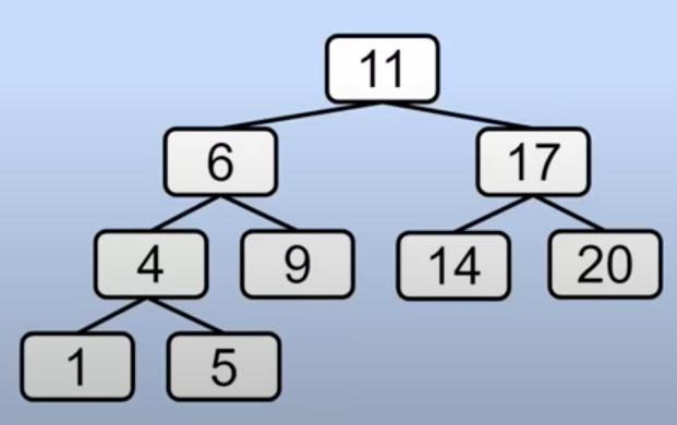
- Not all data can be compared along one dimension
- number and strings can, but what about 2D points?
- Image we have an astronomical image
- What are all the stars within this region?
- What star is closest to the space cat?
- We could iterate over all the objects, but want to be more efficient
- Try to build BST of 2D points
- Simple dataset: Mars at (1.0, 2.8) and Earth at (1.5, 1.6)
- Need to decide how one item is less than another
- Use the x
- Use the y
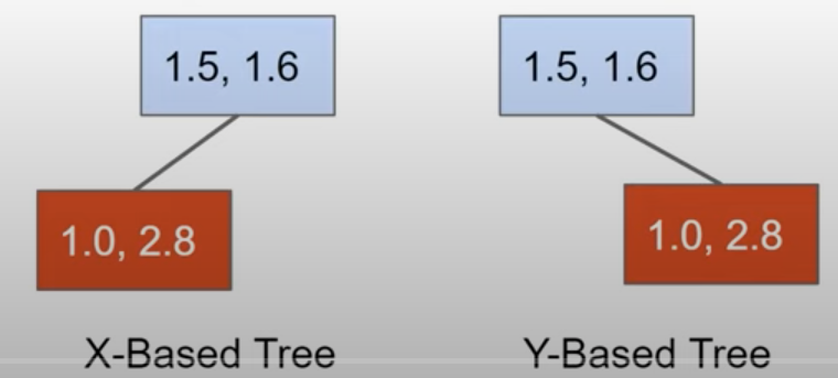
- Consider this example, what would the trees look like
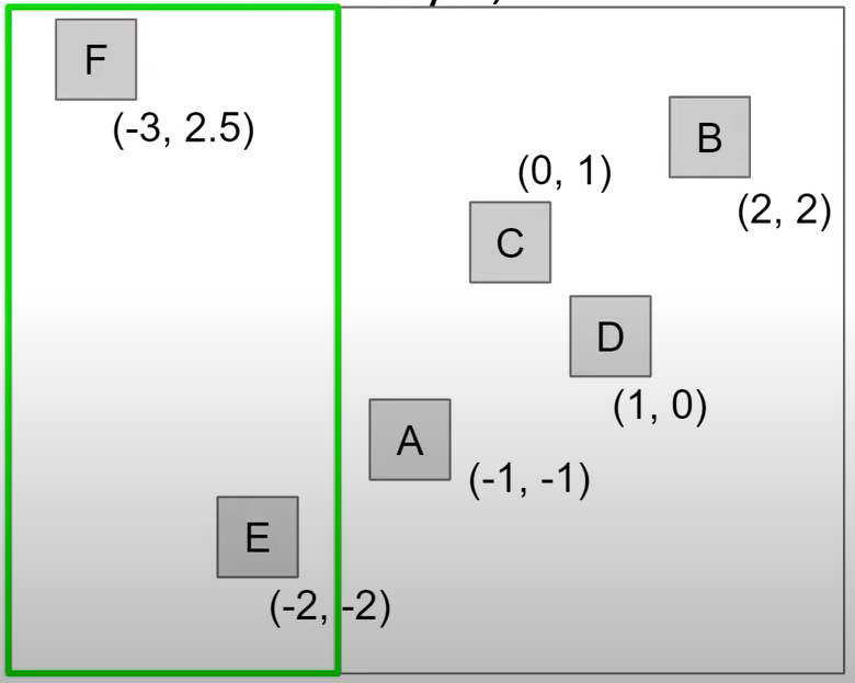
- To find all points with x-coordinate less then -1.5, what would we do
- When tree arranged by x-coordinate, we can prune
- Nodes divide the space of possible nodes into two parts
- Higher dimensional data could be 2D or 3D points, or attributes of a song (length, tempo, popularity, recording date, etc.)
- Common solution: the k-d tree, where k is the number of dimensions
- We'll focus on 2D data (i.e., a 2-d tree)
- Useful data structure, but not one that standard libraries provide
- Common solution: the k-d tree, where k is the number of dimensions
- 2-d tree nodes alternate which coordinate they sort by
- root splits by x, depth 1 nodes split by y, depth 2 nodes split by x, etc.
- https://docs.google.com/presentation/d/1t79IlSaJeOQ1Oau5Y0F8AIO0nlc9_pnuoYxTelCxPV4/edit?usp=sharing
- https://docs.google.com/presentation/d/1sTF3AWHqTNfE3TZX9T0kOy85E9XmvbBNTPoetCfGa4M/edit?usp=sharing
- Applications
- Starlings murmurate:
- Real starlings: https://www.youtube.com/watch?v=eakKfY5aHmY
- Simulated starlings: https://www.youtube.com/watch?v=nbbd5uby0sY
- Efficient simulation means "birds" have to find their nearest neighbors efficiently.
- NBody simulation
- Every object has to calculate the force from every other object.
- This is very silly if the force exerted is small, e.g. individual star in the Andromeda galaxy pulling on the sun.
- One optimization is called Barnes-Hut. Basic idea:
- Represent universe as a k-d tree of objects.
- If a node is sufficiently far away from X, then treat that node and all of its children as a single object.
- Example: Andromeda is very far away, so treat it as a single object for the purposes of force calculation on our sun.
- Starlings murmurate:
3 Practice Problems1
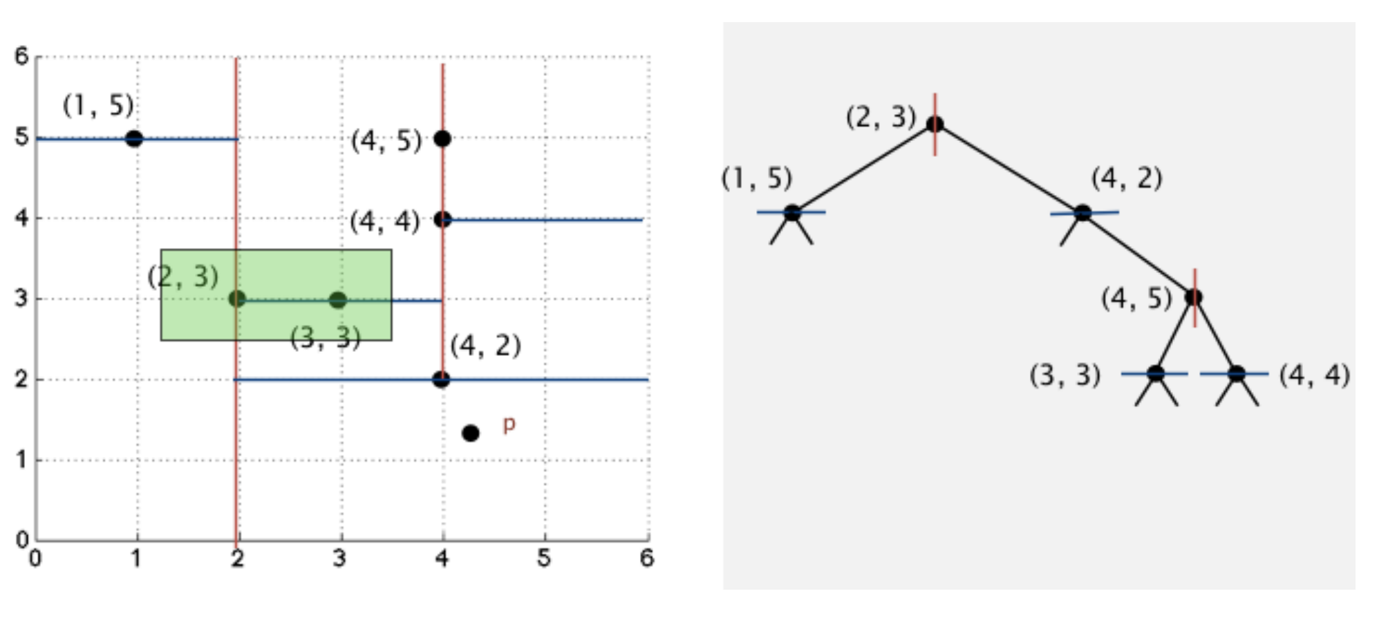
- To the right of the axis below, draw the k-d Tree after inserting the points [(2, 3), (4,2), (4, 5), (3, 3), (1, 5), (4, 4)]. Be careful when inserting (4, 4), as ties are treated the same as greater than. On the axes, draw each point as well as the red or blue lines that bisect the plane through each point.
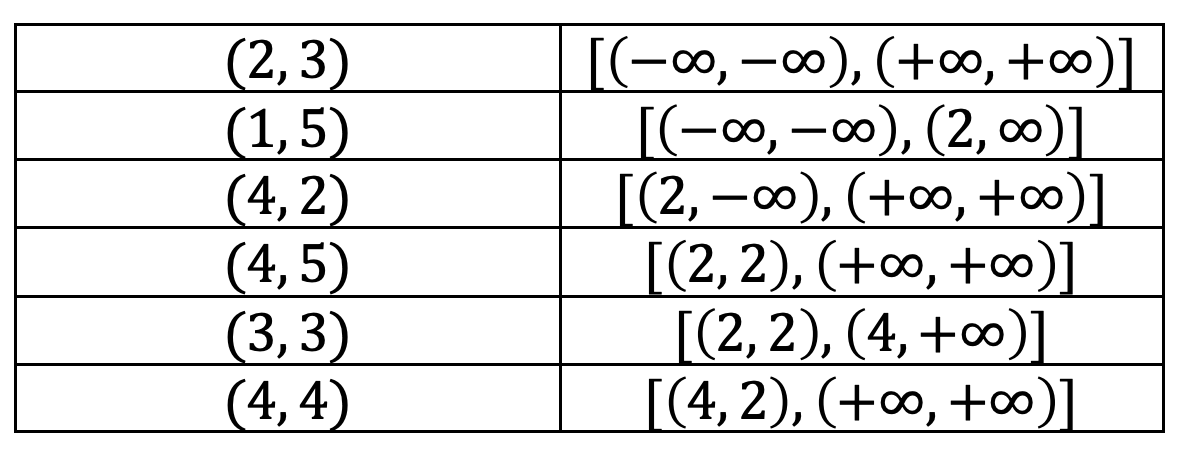
- List the corresponding axis-aligned rectangles for each point. The corresponding axis-aligned rectangle of (2, 3) is [(−∞, −∞), (+∞, +∞)].
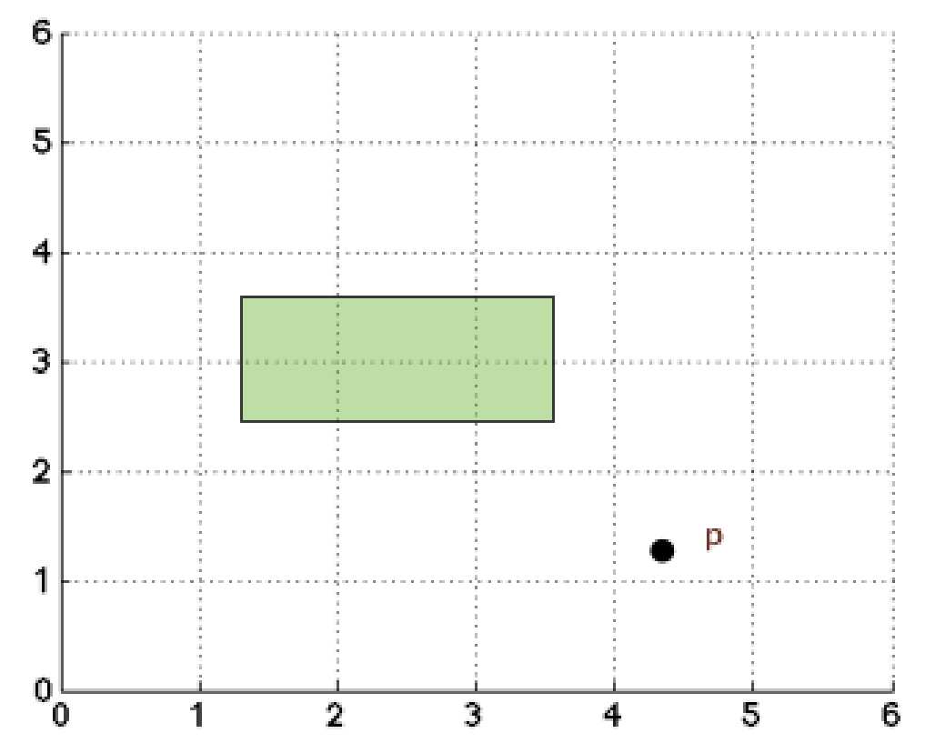
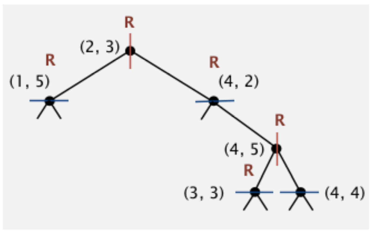
- Consider a range query on the shaded rectangle. Write "R" next to each node in your k-d Tree that is traversed by the range search algorithm. Do not count null nodes or nodes whose corresponding rectangles do not intersect the query rectangle.
- Consider a nearest neighbor query on point p. Number each node (starting with 0) by the order in which it is visited by the nearest neighbor algorithm UNLESS that node's corresponding rectangle rules out that node or its children. For nodes that are pruned based on rectangle distance, write an "X" instead of a number. Do not number null nodes.
Footnotes:
Solutions:
- Geometric and tree representations:
- Table of rectangles:
A nice way to think about (3, 3) for example, is that it is:
- To the right of (2, 3)
- Above (4, 2)
- To the left of (4, 5)
Naturally, this means its corresponding rectangle should be [(2, 2), (4, +∞)]
- Labeled tree:
- Labeled tree:
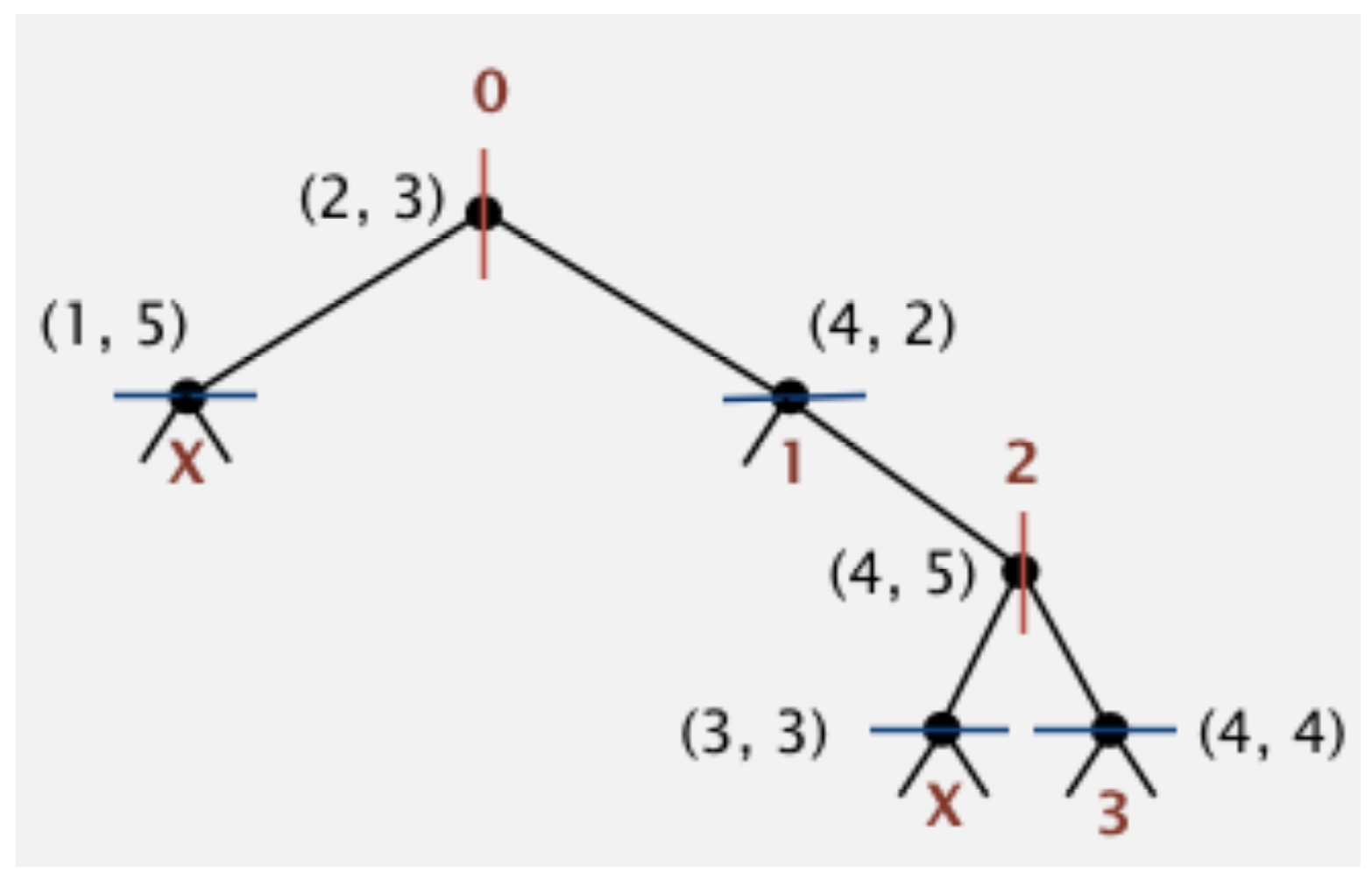
Xs denote nodes that were ruled out. An important point to make here is that the way that we know that (3, 3) and all of its children are farther from the query point is that (3, 3)'s corresponding rectangle is farther from the query point than our current best point (4, 2). The same idea holds true for (1, 5)'s corresponding rectangle, whose distance to p is greater than (4, 2) to p.
Detailed algorithm trace for range search:
- (2, 3): Base case: Check to see if (2, 3)'s corresponding rectangle intersects the green rectangle. Since the (2, 3)'s rectangle is the entire universe, of course it intersects. Check to see if (2, 3) is contained in the rectangle. It is, so add it to the iterable. Go left first (order doesn't matter). We reach (1,5).
- (1, 5): Base case: Check to see if (1, 5)'s corresponding rectangle intersects the green rectangle. Yes, the left half of the bisected plane does indeed intersect, so we proceed. We see if (1, 5) is contained in the green rectangle. It is not. We recur left.
- Null to the left of (1, 5): Base case detects null, returns to (1, 5). This repeats for the right child.
- (4, 2): Corresponding rectangle intersects, so proceed. Point is not part of rectangle. Recur left, is null, return. Recur right.
- (4, 5): Rectangle intersects, so proceed. Point is not part of rectangle. Recur left.
- (3, 3): Rectangle intersects, so proceed. Point is part of rectangle, so add to iterable. Left and right recursive calls result in nulls. Return back to (4, 5), recur right.
- (4, 4): Rectangle for (4, 4) does NOT intersect green rectangle, so abort search. Return to (4, 5). Return to (4, 2). Return to (2, 3). We are done.
Detailed algorithm trace for nearest neighbor:
- Champion point starts as (2, 3). Best distance is also recorded for convenience. Program begins.
- (2, 3): We compute the distance between (2, 3)'s rectangle and the query point, which is 0 since it is contained in the rectangle. 0 is closer than the best distance, so we do not prune. Now we must decide whether to go left or right. We compare (2, 3)'s x coordinate with p's x coordinate. Since p is to the right, we go right first.
- (4, 2) We compute the distance between (4, 2)'s rectangle and the query point, which is again 0. 0 is less than the champion distance, so we do not prune. (4, 2) is closer to the query point than (2, 3), so we make (4, 2) the new champion. We decide to go either up or down. Since p is below (4, 2), we go down first.
- null to the left of (4, 2): Since this is null, we just return. Then we go up from (4, 2).
- (4, 5): The distance between (4, 5)'s rectangle and the query point is something slightly less than 1. This distance is clearly a bit less than the champion distance, so we do not prune. We compare (4, 5)'s distance to p with the champion distance, and it is farther, so (4, 2) remains the champion. We then decide to go left or right. Since p's x coordinate is greater than (4, 5), we go right first.
- (4, 4). The distance from (4, 4)'s rectangle is exactly the same as the previous iteration, just a bit less than 1. This distance is less than the champion distance, so we do not prune. (4, 4)'s distance is farther than the champion distance, so (4, 2) remains the champion. We then decide whether to go down or up. We go down first, see null. Then go up. See null. Then return to (4, 5). Then we go left to (3, 3).
- (3, 3). This point's corresponding rectangle is the same distance from the query point than the current champion. Indeed, the champion (4, 2) is exactly the point defining the corresponding rectangle. Thus, we prune this search, since there's no way we can do better. We return to (4, 5), then to (4, 2), and finally back to (2, 3). From there, we go left to (1, 5).
- (1, 5). This point's corresponding rectangle is the left half of the plane, with distance of a bit more than 2 from the query point. Since this is greater than the champion distance, we prune the search. We return to (2, 3) and we are done.