Lab 2021-04-30: Testing and Query Plans
Table of Contents
1 Query Planning in Postgres
From the documentation:
- generate plans for scanning input tables
- sequential scan always available
- index scans generated if indexes on relevant attributes exist (a predicate or ORDER BY)
- if joins are involved, join plans considered next
- nested loop join
- sort-merge join
- hash join
- Provided the number of joins is under a threshold, the optimizer will try and consider all possible plans, choosing the one with the lowest cost estimate
- Cost estimates depend on a number of constant factors
If you'd like to follow along, download pgAdmin, and create a new server with this information:
- hostname: awb66333.mathcs.carleton.edu
- database: musicbrainz-lab
- username: lab334
- password: strangelove
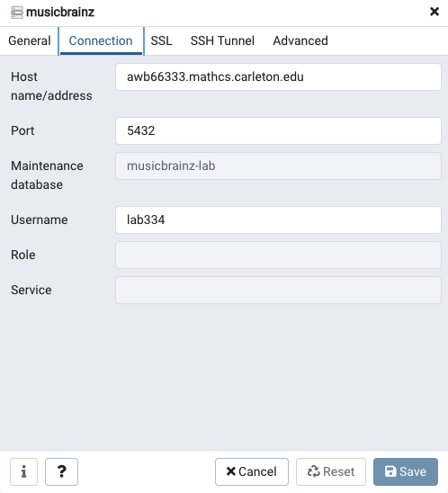
You will need to be on campus or on the Carleton VPN to connect. Go to Tools>Query Tool to bring up a text box where you can enter SQL queries. Use the highlighted buttons to run, explain, and explain analyze your query:

We can use EXPLAIN ANALYZE to have Postgres display the query plan and then execute it and report the actual performance.
1.1 Sorting
musicbrainz=# explain analyze select name from work_type order by name;
Sort  (cost=1.99..2.07 rows=29 width=32) (actual time=0.438..0.440 rows=29 loops=1)
  Sort Key: name
  Sort Method: quicksort  Memory: 26kB
  ->  Seq Scan on work_type  (cost=0.00..1.29 rows=29 width=32) (actual time=0.423..0.426 rows=29 loops=1)
Planning Time: 1.216 ms
Execution Time: 0.451 ms
This shows the query plan as a tree, with each node being an operator (e.g., Seq Scan) followed by the planner's cost estimate, and then the actual performance when the query ran. Indentation indicates parent-child relationships within in the plan. So the above plan does a sequential scan on work_type, and passes the result to its parent, which performs and in-memory quicksort. The work_type table is pretty small (just 29 tuples), so what happens when we sort something bigger?
musicbrainz=# explain analyze select name from artist order by name;
Gather Merge  (cost=106740.32..270375.58 rows=1402490 width=13) (actual time=1139.362..1599.456 rows=1682989 loops=1)
  Workers Planned: 2
  Workers Launched: 2
  ->  Sort  (cost=105740.30..107493.41 rows=701245 width=13) (actual time=1129.528..1261.987 rows=560996 loops=3)
        Sort Key: name
        Sort Method: external merge  Disk: 13728kB
        Worker 0:  Sort Method: external merge  Disk: 12816kB
        Worker 1:  Sort Method: external merge  Disk: 13080kB
        ->  Parallel Seq Scan on artist  (cost=0.00..25663.45 rows=701245 width=13) (actual time=0.165..834.239 rows=560996 loops=3)
Planning Time: 10.243 ms
Execution Time: 1686.454 ms
Two things happened: Postgres switched to an external merge sort, and used two additional threads. If we want to only see sequential plans, we can set the maximum additional workers to 0:
musicbrainz=# SET max_parallel_workers_per_gather = 0;
SET
musicbrainz=# explain analyze select name from artist order by name;
Sort  (cost=267049.78..271257.26 rows=1682989 width=13) (actual time=1259.439..1614.521 rows=1682989 loops=1)
  Sort Key: name
  Sort Method: external merge  Disk: 39544kB
  ->  Seq Scan on artist  (cost=0.00..35480.89 rows=1682989 width=13) (actual time=0.519..240.351 rows=1682989 loops=1)
Planning Time: 0.050 ms
Execution Time: 1711.787 ms
So what determines when Postgres can use quicksort vs external merge sort? The amount of memory available to the query.
musicbrainz=# show work_mem;
 work_mem
----------
 4MB
We can actually modify this variable
musicbrainz=# set work_mem='200MB';
which will give us enough space to sort artist in memory (in this case only a little faster than the external sort):
musicbrainz=# explain analyze select name from artist order by name;
 Sort  (cost=209523.78..213731.26 rows=1682989 width=13) (actual time=1049.520..1348.402 rows=1682989 loops=1)
   Sort Key: name
   Sort Method: quicksort  Memory: 140282kB
   ->  Seq Scan on artist  (cost=0.00..35480.89 rows=1682989 width=13) (actual time=0.027..213.590 rows=1682989 loops=1)
 Planning Time: 0.048 ms
 Execution Time: 1448.885 ms
1.2 Aggregation
musicbrainz=# explain analyze select type, max(length(name)) as m from work group by type;
HashAggregate  (cost=35879.71..35880.00 rows=29 width=12) (actual time=419.469..419.474 rows=30 loops=1)
  Group Key: type
  Batches: 1  Memory Usage: 24kB
  ->  Seq Scan on work  (cost=0.00..25747.12 rows=1351012 width=31) (actual time=0.163..138.471 rows=1351012 loops=1)
Planning Time: 0.145 ms
Execution Time: 419.536 ms
Postgres will typically use HashAggregate for aggregation. If the input to the aggregation will already be sorted, it may use GroupAggregate, which leverages the sorted order to perform aggregation. Tuples coming from an index scan, for example, will be sorted:
CREATE INDEX ix_release_artist_credit ON release (artist_credit);
musicbrainz=# explain analyze select artist_credit, max(length(name)) from release group by artist_credit;
GroupAggregate  (cost=0.43..183426.45 rows=76284 width=12) (actual time=148.184..3878.211 rows=676174 loops=1)
  Group Key: artist_credit
  ->  Index Scan using ix_release_artist_credit on release  (cost=0.43..163230.65 rows=2591062 width=29) (actual time=0.048..3273.448 rows=2591062 loops=1)
Planning Time: 0.279 ms
Execution Time: 3915.244 ms
1.3 Joins
musicbrainz=# explain analyze select area.name, artist.name from artist, area where artist.area = area.id;
Hash Join  (cost=4115.44..74141.46 rows=781692 width=24) (actual time=54.811..549.966 rows=781077 loops=1)
  Hash Cond: (artist.area = area.id)
  ->  Seq Scan on artist  (cost=0.00..35480.89 rows=1682989 width=21) (actual time=0.113..257.758 rows=1682989 loops=1)
  ->  Hash  (cost=1944.42..1944.42 rows=118242 width=19) (actual time=54.620..54.621 rows=118242 loops=1)
        Buckets: 65536  Batches: 2  Memory Usage: 3700kB
        ->  Seq Scan on area  (cost=0.00..1944.42 rows=118242 width=19) (actual time=0.022..16.805 rows=118242 loops=1)
Planning Time: 0.168 ms
Execution Time: 589.453 ms
Here we see Postgres creating a hash table for the smaller relation (area) and then probing it with tuples from artist in order to compute a hash join.
musicbrainz=# explain analyze select area.name, artist.name from artist, area where artist.area = area.id and begin_date_year > 1850;
Hash Join  (cost=4115.44..51570.56 rows=163317 width=24) (actual time=54.630..312.728 rows=298134 loops=1)
  Hash Cond: (artist.area = area.id)
  ->  Seq Scan on artist  (cost=0.00..39688.36 rows=351622 width=21) (actual time=0.039..174.289 rows=350516 loops=1)
        Filter: (begin_date_year > 1850)
        Rows Removed by Filter: 1332473
  ->  Hash  (cost=1944.42..1944.42 rows=118242 width=19) (actual time=54.521..54.522 rows=118242 loops=1)
        Buckets: 65536  Batches: 2  Memory Usage: 3700kB
        ->  Seq Scan on area  (cost=0.00..1944.42 rows=118242 width=19) (actual time=0.013..16.910 rows=118242 loops=1)
Planning Time: 3.462 ms
Execution Time: 328.252 ms
Note how the filter is applied prior to the join.
We know the sort-merge join is best when the incoming data is already sorted. Like with aggregations, this can happen when the data comes from an index:
CREATE INDEX ix_artist_area ON artist (area);
explain analyze select area.name, Count(*) as count
from artist, area
where artist.area = area.id
group by area.name;
HashAggregate  (cost=89201.13..97728.57 rows=89373 width=19) (actual time=363.026..364.495 rows=9153 loops=1)
  Group Key: area.name
  Planned Partitions: 4  Batches: 1  Memory Usage: 2321kB
  ->  Merge Join  (cost=14337.10..39123.99 rows=781692 width=11) (actual time=70.926..240.126 rows=781077 loops=1)
        Merge Cond: (area.id = artist.area)
        ->  Sort  (cost=14332.63..14628.23 rows=118242 width=19) (actual time=70.906..83.606 rows=118209 loops=1)
              Sort Key: area.id
              Sort Method: external merge  Disk: 3848kB
              ->  Seq Scan on area  (cost=0.00..1944.42 rows=118242 width=19) (actual time=0.024..16.356 rows=118242 loops=1)
        ->  Index Only Scan using ix_artist_area on artist  (cost=0.43..31065.26 rows=1682989 width=8) (actual time=0.016..63.098 rows=781078 loops=1)
              Heap Fetches: 0
Planning Time: 0.846 ms
Execution Time: 370.002 ms
2 Testing
- unit tests: small tests as targeted as possible
- make sure everything is called
- try and isolate functions, not always possible
- check return values
- "workload" tests: simulate actual use
- how will the buffer pool be used by the database?
- what challenging situations might arise?
- integrated tests: tests that use all of an object's methods
- check for bugs where calling a method interferes with future calls to other methods
- not found by unit tests
- check for bugs where calling a method interferes with future calls to other methods
2.1 Logging
- When something is going wrong, it's easy to spend hours staring at your code, convincing yourself that it's correct
- Thinking through the code line-by-line can be helpful, but has strongly diminishing returns
- Many potential sources of errors, may be subtle
- e.g., one part of the code makes a faulty assumption about another
- The trusty print statement can come to the rescue (or
LOG_INFO(FORMAT_STRING, ARGS)in the case of bustub) - But what to print?
- Key idea: you want to be able to watch the state of the system evolve
- So things that make changes to this state are useful to log:
LOG_INFO("Unpinning page %d, is_dirty=%d", page_id, is_dirty);LOG_INFO("Fetching page %d", page_id);LOG_INFO("Writing page %d to disk", page_id);LOG_INFO("Allocated new page %d", page_id);