Programming Problem Set #2
You must complete four problems in any combination of numbered exercises and challenges. Check-ins will begin around 20:00 the night the problem set is due.
Starter files available here. Download them, right-click on the zip file, and select “Extract All” to unzip. Then open the programming-2-starter folder in VS Code.
Open a terminal in VSCode (Terminal->New Terminal), paste in the following command, and hit enter.
python -m pip install numpy matplotlib astropy vpython --no-warn-script-locationIf you’re getting errors with files not being found when running your code, there is a VS Code setting you can change that will probably fix them.
Go to File->Preferences->Settings and enter
python.terminal.executeInFileDir in the search box at the
top. A single setting should come up that looks like this:
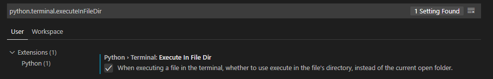
Check that box, and you should be good to go.
Background
In these exercises you will apply your knowledge of lists and loops to the task of image processing. First, some background. You can think of a digital image as a large two-dimensional array of pixels, each of which has a red (R) value, a green (G) value, and a blue (B) value. An R, G, or B value is just decimal number between 0 and 1. To modify the image, you need to loop through all of these pixels, one at a time, and do something to some or all of the pixels. For example, to remove all of the green color from each pixel:for every row in the image:
for every column in the image:
set to zero the green value of the pixel in this row and this column The files for this lab are contained in programming-2-starter.zip. Download and unzip it to get started. These files are
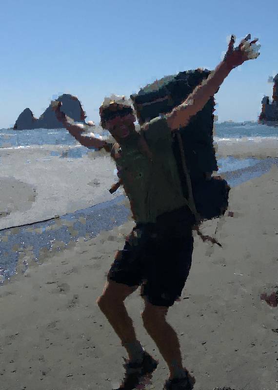
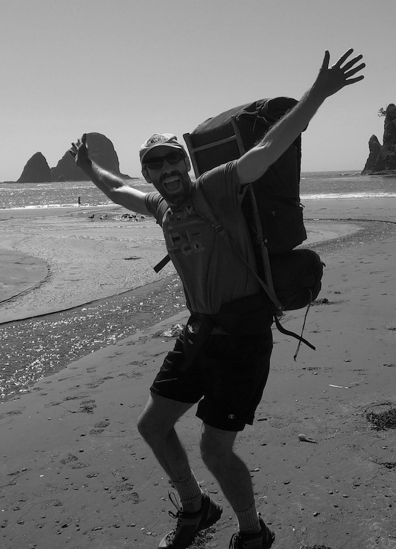
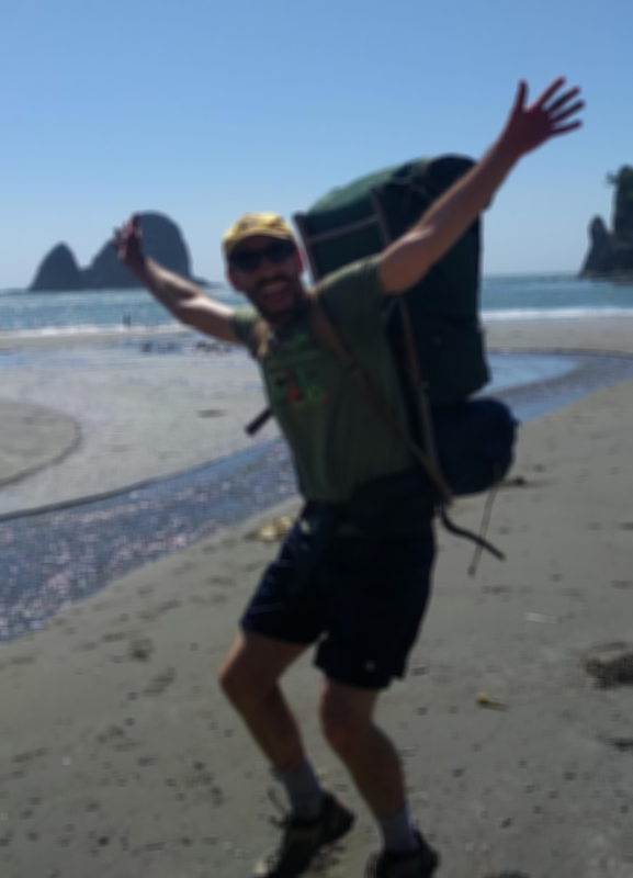
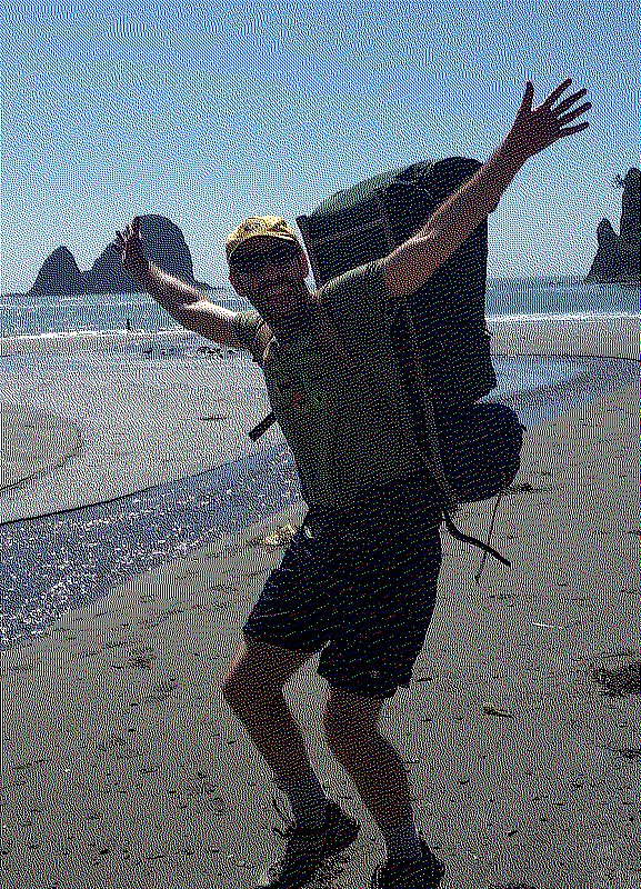
fruit.py: you will modify this file to implement your solution to exercise 0 (Fruit Ninja Academy)gray.py: you will modify this file to implement your solution to exercise 1 (Grayscale)blue_screen.py: you will modify this file to implement your solution to exercise 2 (Blue Screening)blur.py: you will modify this file to implement your solution to exercise 3 (Blur)beach_portrait.png: a picture of some backpacking goofball, used as the input image forgray.pyoz_bluescreen.png: a still photo from the set of the 2013 film Oz the Great and Powerful, used as one of the input images forblue_screen.pymeadow.png: a peaceful meadow scene, used as one of the input images forblue_screen.pyreference-beach_portrait_gray.png: the expected output image forgray.py, provided for your referencereference-oz_meadow.png: the expected output image forblue_screen.py, provided for your referencereference-beach_portrait_blur.png: the expected output image forblur.py, provided for your reference
There are additional files related to the optional challenges as well.
0. Fruit Ninja Academy
Congratulations! The time has come for your final exam at the Fruit
Ninja Academy. The array of fruits you will use to demonstrate your
slicing prowess has already been assembled in the starter code. You will
now face a series of slicing challenges. Extend the provided
fruit.py to accomplish the following tasks, printing out
the result of each task. The expected number of commands (not
necessarily including printing) and expected output are given for each
task.
- Extract the bottom right element in one command.
Tomato- Extract the inner 2x2 square in one command.
[['Grapefruit' 'Kumquat']
['Orange' 'Tangerine']]- Extract the first and third rows in one command.
[['Apple' 'Banana' 'Blueberry' 'Cherry']
['Nectarine' 'Orange' 'Tangerine' 'Pomegranate']]- Extract the inner 2x2 square flipped vertically and horizontally in one command.
[['Tangerine' 'Orange']
['Kumquat' 'Grapefruit']]- Swap the first and last columns in three commands. Hint: make a copy
of an array using the
copy()method.
[['Cherry' 'Banana' 'Blueberry' 'Apple']
 ['Mango' 'Grapefruit' 'Kumquat' 'Coconut']
 ['Pomegranate' 'Orange' 'Tangerine' 'Nectarine']
['Tomato' 'Raspberry' 'Strawberry' 'Lemon']]- Replace every element with the string
"SLICED!"in one command.
[['SLICED!' 'SLICED!' 'SLICED!' 'SLICED!']
 ['SLICED!' 'SLICED!' 'SLICED!' 'SLICED!']
 ['SLICED!' 'SLICED!' 'SLICED!' 'SLICED!']
 ['SLICED!' 'SLICED!' 'SLICED!' 'SLICED!']]
1. Grayscale
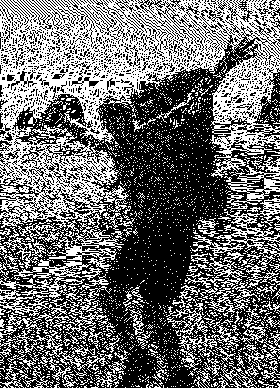
Modify gray.py to convert image to a
black-and-white or grayscale version of the original. In the
RGB color model, gray tones are produced when the values of red, green,
and blue are all equal. A simple way to do this conversion is to set the
red, green, and blue values for each pixel to the average of those
values in the original image. That is \(R_{gray} = G_{gray} = B_{gray} = \frac{R + G +
B}{3}\). When you have implemented a correct solution, running
gray.py should produce a file called
beach_portrat_gray.png that is the same image as
reference-beach_portrait_gray.png:
2. Blue Screening
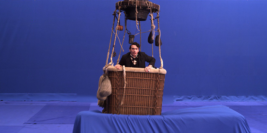
Movies–particularly (non-animated) action movies that use a lot of special effects–often use a technique called blue screening to generate some scenes. The actors in a scene are filmed as they perform in front of a blue screen and, later, the special-effects crew removes the blue from the scene and replaces it with another background (an ocean, a skyline, the Carleton campus). The same technique is used for television weather reports–the meteorologist is not really gesturing at cold fronts and snow storms, just at a blank screen. (Sometimes green screening is used instead; the choice depends on things like the skin tone of the star.) This problem asks you to do something similar.
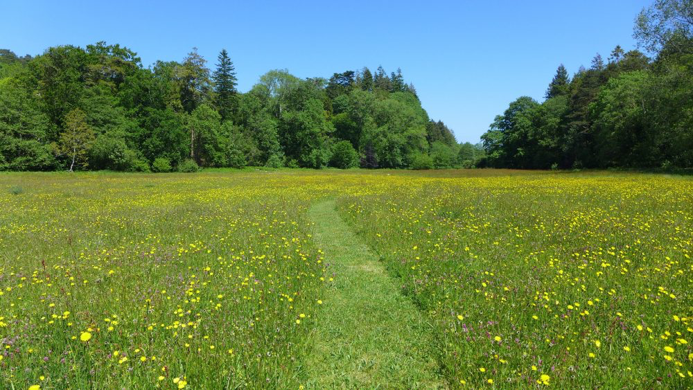
We can combine an image of, say, James Franco on the set of
Oz the Great and Powerful (oz_bluescreen.png) with
an image of scenery (meadow.png) by replacing the bluish
pixels in the first picture with pixels from a background picture. To do
this, we have to figure out which pixels are bluish (and can be changed)
and which ones correspond to the actor and props (and should be left
alone). Identifying which pixels are sufficiently blue is tricky. Here’s
an approach that works reasonably well here: count any pixel that
satisfies the following formula as “blue” for the purposes of blue
screening: \(B > R + G\).
Modify blue_screen.py to use this formula to replace the
appropriate pixels in image with pixels from
background. When you have implemented a correct solution,
running blue_screen.py should produce a file called
oz_meadow.png that is the same image as
reference-oz_meadow.png.
 +
+
 =
=

3. Blur
Modify blur.py to implement the function
blur(img, radius). Your blur function should
create and return a blurry version of the image (img). For
each pixel, average all of the pixels within a square
radius of that pixel. Here’s an example what that
means:
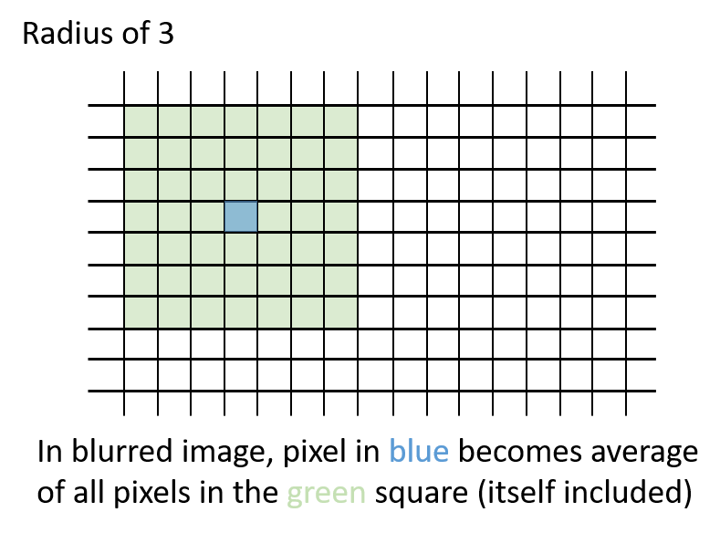
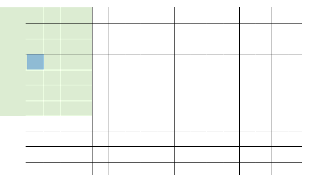
Each pixel will become the average of the square of pixels around it. Pixels at the edges of the image will use whatever part of the square actually exists. Here’s an animation of how the square radius moves with each pixel:
A good way to approach this would be to use radius to
slice out a square around the pixel in question. For example,
img[0:10, 0:10] would slice out a 10-by-10 square from the
upper left corner of the image (note that unlike lists,
arrays let us index rows and columns separated by commas
instead of multiple sets of brackets). To get the average of the
elements of an array you can use .mean()
(e.g., img[:, :, 0].mean() would be the average red value
for the entire image because it slices out all rows, all columns, and
the first element (red) of each pixel).
Make sure to put all of your results in a new image
(img.copy() will return a copy of img),
instead of overwriting your original as you go; otherwise, your blurred
pixels will cascade on top of each other. Be careful near the borders of
the image. Keep in mind that some approaches to this problem will result
in much slower performance. Any technique that works will receive most
of the credit, but your blur.py should run in less than 30
seconds to earn full credit. But do be careful; it’s possible to find
solution that take a lot longer!
When you have implemented a correct solution, running
blur.py should produce a file called
beach_portrait_blur.png that is the same image as
reference-beach_portrait_blur.png. Make sure your code
calls blur with a radius of 3 like the starter code.
Challenges
C1. Dithering
Dithering is a technique often used to print a gray picture in a legacy medium (such as a newspaper) where no shades of gray are available. Instead, you need to use individual pixels of black and white to simulate shades of gray. A standard approach to dithering is the Floyd–Steinberg algorithm, which works as follows:
- Loop over all pixels as always, from top to bottom and, within each row, from left to right.
- For each pixel: if its value is larger than 0.5, then set it to 1.0 (pure white). Otherwise, set it to 0 (pure black). Since this is a grayscale image, the red, green, and blue channels will all be equal. Record the error, which represents how much blackness we have added to this pixel, by taking the old value of this pixel minus the new one. Note that the error can be positive or negative, depending on whether you adjusted the color blackwards or whitewards.
- Distribute this pixel’s error to adjacent pixels as follows:
- Add 7/16 of the error to the pixel immediately to the right (“east”).
- Add 3/16 of the error to the pixel immediately diagonally to the bottom left (“southwest”).
- Add 5/16 of the error to the pixel immediately below (“south”).
- Add 1/16 of the error to the pixel immediately diagonally to the bottom right (“southeast”). Be careful near the edges of the image! If some error should be distributed to a pixel that doesn’t exist (e.g., it’s off the edge of the image), you should just ignore that part of the error.
Some tips: (1) while dithering can be used with color images, it’s
more complicated, so start by using gray.py to convert an
image to gray before you get started. (2) In order for dithering to
work, you must make your changes to the same image that you are looping
over. Dithering by reading one image and making your changes on a copy
will not work correctly, because the error never gets a chance
to accumulate. In other words, make sure that you make a grayscale copy
of the image first, and then do all dithering work (looping, reading,
writing, etc.) on the copy itself.
Now that you have dithering working for grayscale images, extend your dithering function to work for color images as well. It will need to take the desired number of colors per channel (\(n\)) as an argument. For example, if \(n = 2\), then pixels in the dithered image will have one of two possible values for red (0 or 1.0), and similarly for green and blue (for a total of eight possible colors).
To transform a color in the original image to the corresponding dithered color, you’ll need to round the original color to the closest color in the restricted dithered palette. Be sure to apply error separately for each color channel.
An example output image with \(n = 2\):
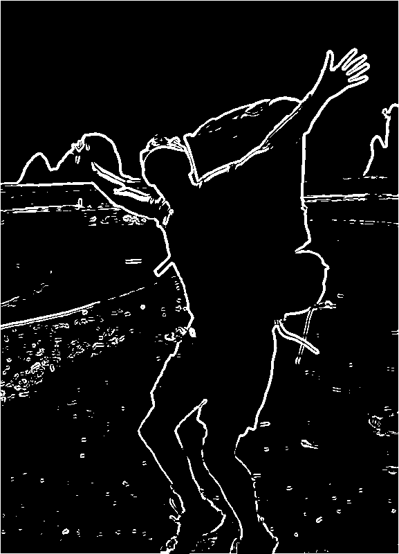
C2. Edge Detection
The Sobel edge detection algorithm highlights the edges of objects in an image. It works by detecting areas with a high variation in pixel values (gradients).
Algorithm
The algorithm consists of three steps:
- Calculate horizontal (\(G_x\)) and vertical (\(G_y\)) gradient values for each pixel in the image.
- Calculate the final gradient magnitude for each pixel using the calculated \(G_x\) and \(G_y\) values.
- Set each pixel to black or white based on whether the magnitude exceeds a user-provided threshold
To compute \(G_x\) and \(G_y\) values, use the following Sobel operator kernels:
\[ G_x = \begin{bmatrix} -1 & 0 & 1 \\ -2 & 0 & 2 \\ -1 & 0 & 1 \end{bmatrix} \]
\[ G_y = \begin{bmatrix} -1 & -2 & -1 \\ 0 & 0 & 0 \\ 1 & 2 & 1 \end{bmatrix} \]
To apply a Sobel operator kernel to a pixel, you must perform a convolution operation. A convolution is the sum of the element-wise multiplication of the kernel with the surrounding pixel values. Then, the final gradient magnitude \(G\) can be calculated as follows:
\[G = \sqrt{G_x^2 + G_y^2}\]
If the input image is in color, you should first convert it to grayscale, as the algorithm works on grayscale images. You might also exploring blurring the input image to reduce the noise in the detected edges.
Make sure to handle border cases, where the Sobel operator kernel may not fit. One solution is to ignore the borders or use edge padding (e.g., mirroring the pixels adjacent to the border).
Expected Output
An example output image with a threshold of 40% of the maximum pixel value and a radius-2 blur applied to the input image:
C3. Mosaic
In this challenge, you will implement an image mosaic operation that selects a random region in the input image and replaces it with the most similar region in the image. The user provides the width and height of the regions to move and the number of moves to perform.
Algorithm
- Load the input image using
plt.imread. - Repeat the number of
movesspecified by the user:- Select a random region in the image with the user-specified
widthandheight. Let’s call itregion1. - Divide the image into a grid of
width-by-heightregions. Let’s call this set of sub-imagestargets. - Search
targetsfor the region (let’s call itregion2) that is the most similar toregion1. Use the mean-squared error (MSE) metric for image similarity. - Swap the pixels of
region1with the pixels ofregion2.
- Select a random region in the image with the user-specified
- Save the modified image using
plt.imsave.
Mean-Squared Error (MSE) Metric
The mean-squared error (MSE) between two equally sized image regions \(A\) (width \(w\), height \(h\)) and \(B\) is defined as:
\[ MSE(A, B) = \frac{1}{w \times h} \sum_{x=1}^w \sum_{y=1}^h (A_{xy} - B_{xy})^2 \]
where \(A_{xy}\) and \(B_{xy}\) are the pixel values at position \((x,y)\) in regions \(A\) and \(B\), respectively. The smaller the MSE value, the more similar the image regions are.
Expected Output
An example output image created by 10,000 moves of 10 pixel-by-10 pixel regions: