Database Storage
Table of Contents
Adapted from Andy Pavlo1
1 Storage
We will focus on a disk-oriented DBMS architecture that assumes that primary storage location of the database is on non-volatile disk. Refer to the notes from last week for an overview of the storage hierarchy.
There is also a new class of storage devices that are becoming more popular called persistent memory. These devices are designed to be the best of both worlds: almost as fast as DRAM with the persistence of disk. We will not cover these devices in this course.
Since the system assumes that the database is stored on disk, the components of the DBMS are responsible for figuring out how to move data between non-volatile disk and volatile memory since the system cannot operate on the data directly on disk.
We will focus on how we can hide the latency of the disk rather than focusing on optimizations with registers and caches since getting data from disk is so slow. If reading data from the L1 cache reference took half a second, reading from an SSD would take 1.7 days, and reading from an HDD would take 16.5 weeks.
2 DBMS vs OS
A high-level design goal of the DBMS is to support databases that exceed the amount of memory available. Since reading/writing to disk is expensive, it must be managed carefully. We do not want large stalls from fetching something from disk to slow down everything else. We want the DBMS to be able to process other queries while it is waiting to get the data from disk.
This high-level design goal is like virtual memory, where there is a large address space and a place for the OS to bring in pages from disk. The OS already has a virtual memory system—could we save ourselves a lot of work and just use that in our DBMS?
The problem is that the OS doesn't know anything about what the DBMS is doing and how it's using memory. While it's possible to give the OS hints via
madvise: Tells the OS know when you are planning on reading certain pages.mlock: Tells the OS to not swap memory ranges out to disk.msync: Tells the OS to flush memory ranges out to disk.
The DBMS (almost) always wants to control things itself and can do a better job at it since it knows more about the data being accessed and the queries being processed. Even though the system will have functionalities that seem like something the OS can provide, having the DBMS implement these procedures itself gives it better control and performance.
3 Database Pages
The DBMS organizes the database across one or more files in fixed-size blocks of data called pages. Pages can contain different kinds of data (tuples, indexes, etc). Most systems will not mix these types within pages.
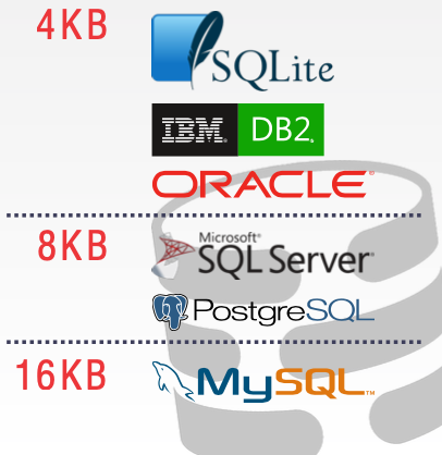
Most DBMSs uses fixed-size pages to avoid the engineering overhead needed to support variable-sized pages. For example, with variable-size pages, deleting a page could create a hole in files that the DBMS cannot easily fill with new pages. There are three concepts of pages in DBMS:
- Hardware page (usually 4 KB).
- OS page (usually 4 KB).
- Database page (512 B-16 KB).
The storage device guarantees an atomic write of the size of the hardware page. If the hardware page is 4 KB and the system tries to write 4 KB to the disk, either all 4 KB will be written, or none of it will. This means that if our database page is larger than our hardware page, the DBMS will have to take extra measures to ensure that the data gets written out safely since the program can get part-way through writing a database page to disk when the system crashes.
3.1 Heap File Organization
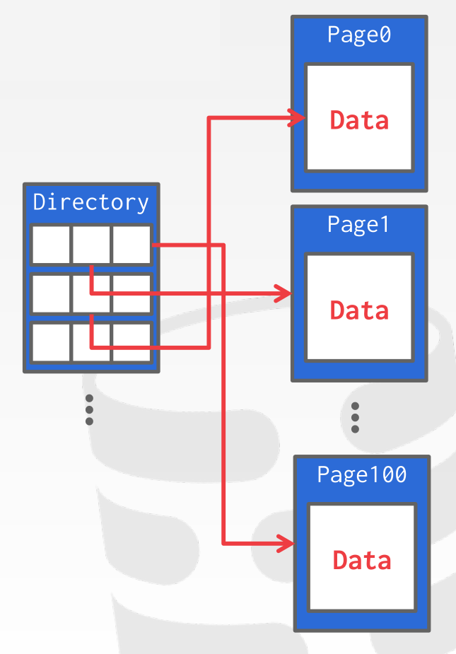
A common way to organize pages on disk is to use a heap file approach. A heap file is an unordered collection of pages where tuples are stored in arbitrary order. The DBMS maintains a page directory that maps a page id to the locations of the page along with the amount of free space it has.
4 Page Layout
Every page includes a header that records meta-data about the page's contents:
- Page size
- Checksum
- DBMS version
- Transaction visibility
A strawman approach to laying out data is to keep track of how many tuples the DBMS has stored in a page and then append to the end every time a new tuple is added. However, problems arise when tuples are deleted or when tuples have variable-length attributes. There are two main approaches to laying out data in pages: (1) slotted-pages and (2) log-structured.
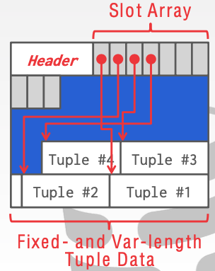
Slotted Pages: Page maps slots to offsets. (Tuple-oriented approach)
- Most common approach used in DBMSs today. (Exact details will vary by system).
- Header keeps track of the number of used slots, the offset of the starting location of the last used slot, and a slot array, which keeps track of the location of the start of each tuple.
- To add a tuple, the slot array will grow from the beginning to the end, and the data of the tuples will grow from end to the beginning. The page is considered full when the slot array and the tuple data meet.
Demo of how different systems organize tuples (Andy Pavlo). Also shows how different systems label tuples internally for the purposes of locating them within the database.2
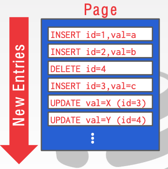
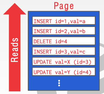
Log-Structured: Instead of storing tuples, the DBMS only stores log records. (Log-oriented approach)
- Stores records of how the database was modified (insert, update, deletes).
- To read data, the DBMS scans the log file backwards and recreates the tuple.
- Fast writes, potentially slow reads.
- Works well on append-only storage because the DBMS cannot go back and update the data.
To avoid long reads, the DBMS can have indexes to allow it to jump to specific locations in the log. It can also periodically compact the log. (If it had a tuple and then made an update to it, it could compact it down to just inserting the updated tuple.) The issue with compaction is that the DBMS ends up with write amplification. (It re-writes the same data over and over again.)
5 Data Representation
The data in a tuple is essentially just byte arrays. It is up to the DBMS to know how to interpret those bytes to derive the values for attributes. A data representation scheme is how a DBMS stores the bytes for a value.
There are five high level datatypes that can be stored in tuples: integers, variable-precision numbers, fixed- point precision numbers, variable length values, and dates/times.
5.1 Integers
Most DBMSs store integers using their native C/C++ types as specified by the IEEE-754 standard. These values are fixed length.
Examples: INTEGER, BIGINT, SMALLINT, TINYINT
5.2 Variable Precision Numbers
These are inexact, variable-precision numeric types that use the native C/C++ types specified by IEEE-754 standard. These values are also fixed length.
Operations on variable-precision numbers are faster to compute than arbitrary precision numbers because the CPU can execute instructions on them directly. However, there may be rounding errors when performing computations due to the fact that some numbers cannot be represented precisely.
Examples: FLOAT, REAL
5.3 Fixed-Point Precision Numbers
These are numeric data types with arbitrary precision and scale. They are typically stored in exact, variable-length binary representation (almost like a string) with additional meta-data that will tell the system things like the length of the data and where the decimal should be. These data types are used when rounding errors are unacceptable, but the DBMS pays a performance penalty to get this accuracy.
Examples: NUMERIC, DECIMAL.
Demo of variable precision vs fixed-point precision (Andy Pavlo)
5.4 Variable-Length Data
These represent data types of arbitrary length. They are typically stored with a header that keeps track of the length of the string to make it easy to jump to the next value. It may also contain a checksum for the data.
Most DBMSs do not allow a tuple to exceed the size of a single page. The ones that do store the data on a special overflow page and have the tuple contain a reference to that page. These overflow pages can contain pointers to additional overflow pages until all the data can be stored.
Some systems will let you store these large values in an external file, and then the tuple will contain a pointer to that file. For example, if the database is storing photo information, the DBMS can store the photos in the external files rather than having them take up large amounts of space in the DBMS. One downside of this is that the DBMS cannot manipulate the contents of this file. Thus, there are no durability or transaction protections.
Examples: VARCHAR, VARBINARY, TEXT, BLOB
5.5 Dates and Times
Representations for date/time vary for different systems. Typically, these are represented as some unit time (micro/milli)seconds since the Unix epoch.
Examples: TIME, DATE, TIMESTAMP
5.6 System Catalogs
In order for the DBMS to be able to decipher the contents of tuples, it maintains an internal catalog to tell it meta-data about the databases. The meta-data will contain information about what tables and columns the databases have along with their types and the orderings of the values.
Most DBMSs store their catalog inside of themselves in the format that they use for their tables. They use special code to "bootstrap" these catalog tables.
6 Workloads
There are many different workloads for database systems. By workload, we are referring to the general nature of requests a system will have to handle. This course will focus on two types: Online Transaction Processing and Online Analytical Processing.
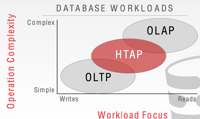
6.1 OLTP: Online Transaction Processing
An OLTP workload is characterized by fast, short running operations, simple queries that operate on single entity at a time, and repetitive operations. An OLTP workload will typically handle more writes than reads.
An example of an OLTP workload is the Amazon storefront. Users can add things to their cart, they can make purchases, but the actions only affect their account.
6.2 OLAP: Online Analytical Processing
An OLAP workload is characterized by long running, complex queries, reads on large portions of the database. In OLAP workloads, the database system is analyzing and deriving new data from existing data collected on the OLTP side.
An example of an OLAP workload would be Amazon computing the five most bought items over a one month period for these geographical locations.
6.3 HTAP: Hybrid Transaction + Analytical Processing
A new type of workload which has become popular recently is HTAP, which is like a combination which tries to do OLTP and OLAP together on the same database.
7 Storage Models
There are different ways to store tuples in pages. We have assumed the n-ary storage model so far, but the relational model doesn't require a particular structure.
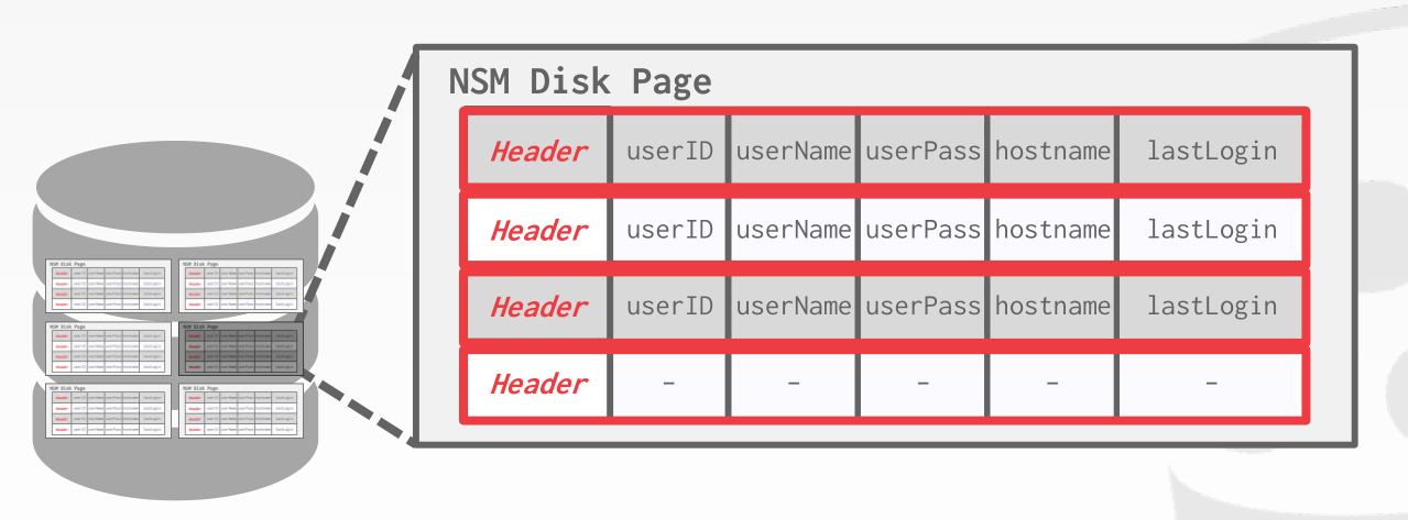
7.1 N-Ary Storage Model (NSM)
In the n-ary storage model, the DBMS stores all of the attributes for a single tuple contiguously in a single page, so NSM is also known as a row store. This approach is ideal for OLTP workloads where requests are insert-heavy and transactions tend to operate only an individual entity. It is ideal because it takes only one fetch to be able to get all of the attributes for a single tuple.
Advantages:
- Fast inserts, updates, and deletes.
- Good for queries that need the entire tuple.
Disadvantages:
- Not good for scanning large portions of the table and/or a subset of the attributes. This is because it pollutes the buffer pool by fetching data that is not needed for processing the query.
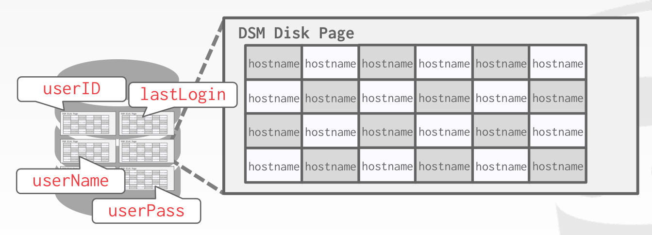
7.2 Decomposition Storage Model (DSM)
In the decomposition storage model, the DBMS stores a single attribute (column) for all tuples contiguously in a block of data. Thus, it is also known as a column store. This model is ideal for OLAP workloads with many read-only queries that perform large scans over a subset of the table's attributes.
Advantages:
- Reduces the amount of wasted work during query execution because the DBMS only reads the data that it needs for that query.
- Enables better compression because all of the values for the same attribute are stored contiguously.
Disadvantages:
- Slow for point queries, inserts, updates, and deletes because of tuple splitting/stitching.
To put the tuples back together when using a column store, there are two common approaches: The most commonly used approach is fixed-length offsets. Assuming the attributes are all fixed-length, the DBMS can compute the offset of the attribute for each tuple. Then when the system wants the attribute for a specific tuple, it knows how to jump to that spot in the file from the offset. To accommodate the variable-length fields, the system can either pad fields so that they are all the same length or use a dictionary that takes a fixed-size integer and maps the integer to the value.
A less common approach is to use embedded tuple ids. Here, for every attribute in the columns, the DBMS stores a tuple id (ex: a primary key) with it. The system then would also store a mapping to tell it how to jump to every attribute that has that id. Note that this method has a large storage overhead because it needs to store a tuple id for every attribute entry.
Footnotes:
The DBMS needs a way to keep track of individual tuples. Each tuple is assigned a unique record identifier.
- Most common: page id + offset/slot
- Can also contain file location info.
An application/database user cannot rely on these ids to mean anything (i.e., they are for internal use only).