Indexes and the B+ Tree
Table of Contents
1 Accessing Data
- Recall we will typically store our data in a heap file (see the topic on database storage)
- Operations will include
- Create or destroy a file
- Insert a tuple
- Delete a tuple with a given record id (RID)
- RID: unique tuple identifier, details vary by system
- Get a tuple with a given rid
- Scan all tuples in the file (a sequential scan)
- But wait there's more!
- We may want to Scan all tuples in the file that match a predicate
- Example: Find all students with GPA > 3.5
- Critical to support such requests efficiently
- Why read all data form disk when we only need a small fraction of that data?
- Today's topic is about how to accomplish this
- We may want to Scan all tuples in the file that match a predicate
1.1 Searching a Heap File
File is not sorted on any attribute
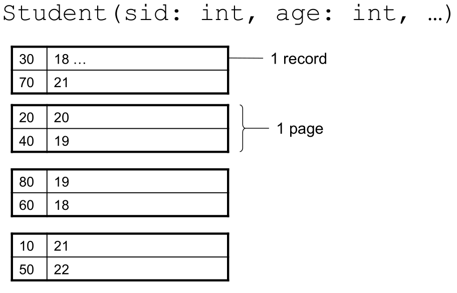
- For example, if there are 10,000 students and 10 student tuples per page
- Total number of pages: 1,000 pages
- Find student whose sid is 80
- Must read on average 500 pages
- Find all students older than 20
- Must read all 1,000 pages
- Can we do better?
2 Sequential File
File sorted on an attribute, usually on primary key
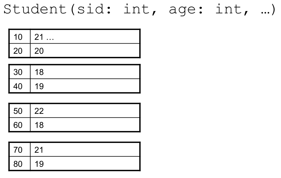
- Total number of pages: 1,000 pages
- Find student whose sid is 80
- Could do binary search, read log2(1,000) ≈ 10 pages
- Find all students older than 20
- Must still read all 1,000 pages
- Can we do even better?
- Note: Sorted files are inefficient for inserts/deletes
3 Indexes
- Index: data structure that organizes data tuples on disk to optimize selections on the search key fields for the index
- An index contains a collection of data entries, and supports efficient retrieval of all data entries with a given search key value k
- The search key can be any set of attributes
- Data entries can be
- (k, RID)
- (k, list-of-RIDs)
- The actual tuple with key k
- We may have multiple indexes for the same data, each organized according to different keys
- A an index of student tuples by age and an index of student tuples by GPA
- Indexes may fit entirely in memory or may be stored as pages on disk just like heap files
- Hash tables can make good in-memory indexes (temporary hash tables are often used as part of join operations)
- Support point queries, but not range queries
- Bad when index doesn't fit in memory, as hashing requires a lot of random-access lookups, which are slow on disk
- Hash tables can make good in-memory indexes (temporary hash tables are often used as part of join operations)
3.1 Clustering vs Nonclustering
- A clustered index is an index where the order of the search keys corresponds to the order of the tuples in the data file
- That is, the data file contains tuples in a sorted order
- Also called a primary index
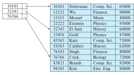
- A clustered index can be dense, meaning it has an entry for every search-key value in the data
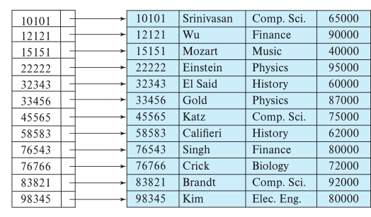
The index can also be sparse, where it has entries for only some of the search-key values
- This necessarily requires the data to be in sorted order of the search key
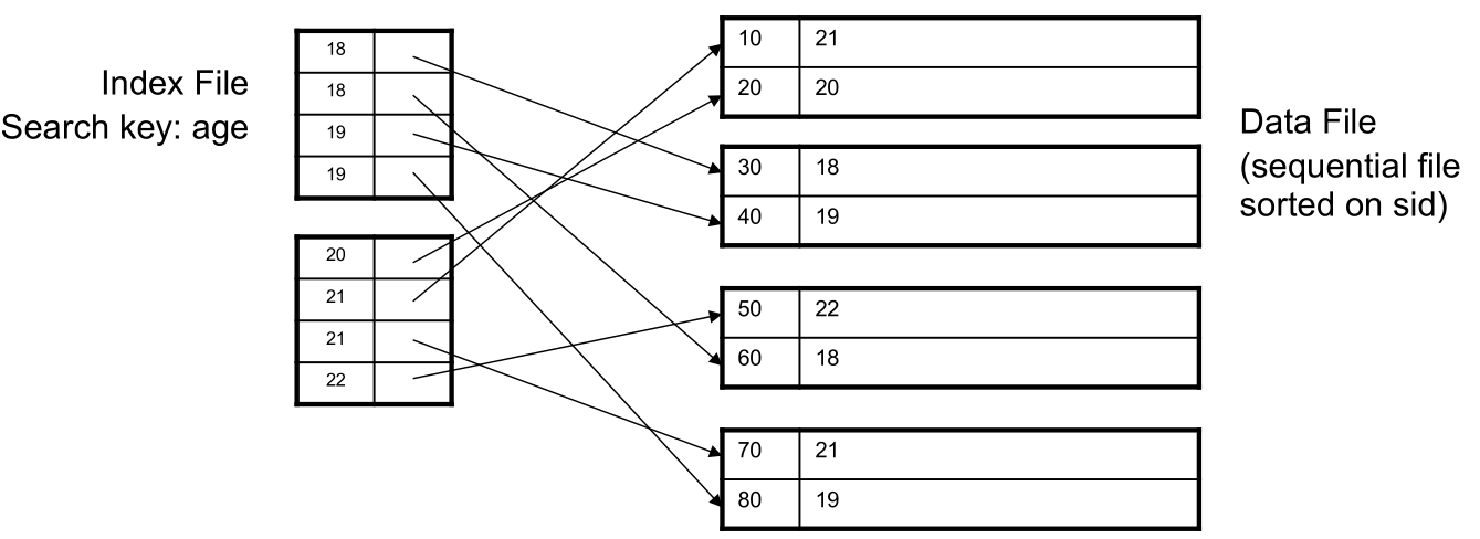
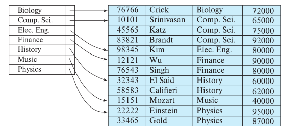
- A clustered index does not have to be on a primary key, as shown here:
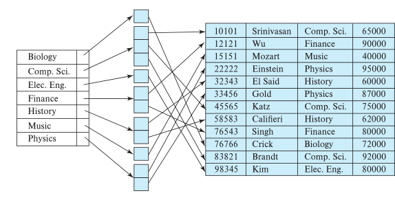
The search keys of a nonclustered index are in a different order than the tuples of the data file
- These must always be dense
- Can see that an index could make a query like "find student who sid is 80" very efficient
- Would only need to read 1 page from disk (the index would point to exactly the page you need)
- What about a "find all students older than 20" query?
- Seems like a clustered index would be useful (i.e., find where to start reading pages on disk)
- But how would we navigate the index? How would it handle updates? What if it isn't clustered?
- For sorted files, performance degrades as the file grows, both for index lookups and for sequential scans through the data
- We need a flexible and robust index data structure
4 B+ Trees
- The B+ Tree is the most common index data structure in database systems
- The inventors of the original B-Tree structure have never explained what the B stands for
- Boeing (where the inventors worked), balanced, broad, bushy, and Bayer (one of the inventors) have all been suggested
- Inventor Edward McCreight has said "the more you think about what the B in B-trees means, the better you understand B-trees."
- The inventors of the original B-Tree structure have never explained what the B stands for
- It has several important properties:
- Perfectly balanced search tree (all leaf nodes are the same depth)
- It generalizes the binary search tree from two children to \(M\) children
- Where \(M\) is a fixed constant for any particular B+ Tree
- Every inner node other than the root must be at least half capacity (has \(m\) children where \(\lceil M/2\rceil \le m \le M\))
- Every inner node with \(m\) children has \(m - 1\) keys
- Every leaf node must be at least half full (holds \(k\) keys where \(\lceil (M-1)/2\rceil \le k \le M - 1\))
- Insert and delete operations will rebalance the tree to maintain these properties
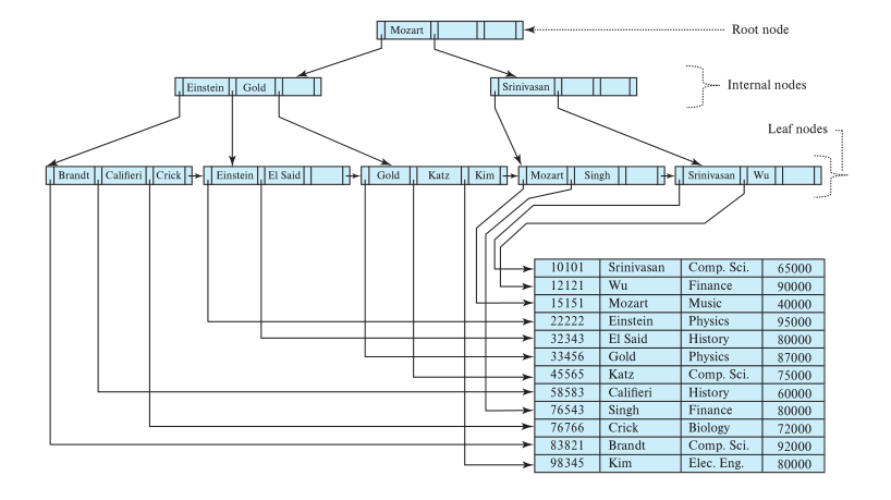
An example of a b+ Tree where \(M = 4\)
4.1 Node Structure
- Every B+ Tree node is comprised of an array of key/value pairs.
- The keys are derived from the attributes(s) that the index is based on.
- The values will differ based on whether the node is classified as inner nodes or leaf nodes.
- For inner nodes, the values are pointers to child nodes
- i.e., inner nodes do not store any actual data, just guide the search to the leaf nodes
For leaf nodes, the values are the index values (RID, list of RIDs, or entire tuples)
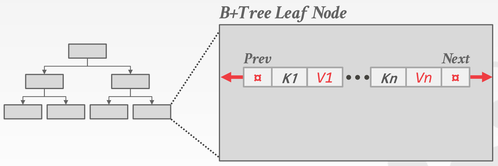
- Leaf nodes also have pointers to their siblings (prev, next in the diagram)
- Faciliates efficient range queries by scanning along leaf nodes without having to re-traverse the tree
- For inner nodes, the values are pointers to child nodes
- The arrays are (usually) kept in sorted key order.
- Each node will be a page
4.2 Insert
See the textbook excerpt for the complete procedure (figures 14.16, 14.17).
- Find the leaf node \(L\) in which you will insert your key
- You can do this by traversing down the tree
- If \(L\) is already full (\(M-1\) entries)…
- Create a new node \(L'\)
- Redistribute the entries, including the new key, evenly between \(L\) and \(L'\)
- Insert the middle key into \(L\)'s parent and add a child pointer to \(L'\)
- The middle key will be the first one in \(L'\)
- If the parent is already full, repeat 2. for the parent
- When splitting inner nodes, the middle key is moved up instead of copied up
4.3 Delete
See the textbook excerpt for the complete procedure (figure 14.18).
- Find the leaf node \(L\) where the key belongs and remove it
- If \(L\) is below half full…
- Try to redistribute, borrowing from sibling (adjacent node with same parent as \(L\))
- If redistribution is not possible, merge \(L\) and sibling
- If merge occurred, delete entry from parent of \(L\) that points to now-merged node
4.4 Examples
- Useful example to work through to make sure you understand insertion and deletion: https://www.cs.nmsu.edu/~hcao/teaching/cs582/note/DB2_4_BplusTreeExample.pdf (Huiping Cao, New Mexico State University)
- Alternative notes from Jenny Huang at UC Berkeley
- Interactive demo: https://goneill.co.nz/btree-demo.php